Maybe you don't need Latex?

If you don’t write a math book, you probably don’t need Latex. Just install LibreOffice, create a document in LibreOffice Writer, then click File - Export as - Export directly as PDF.

That’s all, and you don’t need to:

  1. Install Latex
  2. Install a TON of packages/fonts/language packs for it.
  3. Read answers on latex forums/stackoverflow (stackexcahange) for hours just to be able to generate a PDF file.
  4. Learn unintuitive markup language, time for learning which will never pay off.


Sublime text plugins that work

Essentially my Sublime text setup requires only three things:

  • Terminus - terminal emulator right in the editor. The nice thing is that you can open terminal in a special panel, or you can open a terminal in a new tab.
  • Sublime LSP - LSP support
  • WordingStatus - Shows words count and statistics for a document.


Atom text editor's sunset

"A hackable editor for the 21st Century”, they said.

How it was at the beginning

In 2014-2015 ( I’ve found snapshots of atom.io website for 2014 year on waybackmachine, but Wikipedia says that it was released in 2015), Github released Atom ( I personally can’t recall when I first heard of Atom) - “A hackable editor for the 21st Century”. It quickly became very popular, because… I don’t know why, I never liked it. Anyway, it’s the fact. Atom was a loud name. None of “Best editors for…” types of articles and blog posts hadn’t mentioned Atom as a honorable member of their lists. It was built using web technologies ( that wasn’t so popular as now ), it was free, and a language for its extension was Javascript - one of the most popular languages. Because of electron, Atom was RAM expensive for a text editor ( especially in comparison to Sublime Text, Emacs, Vim or Notepad++ ), but for most users it wasn’t an issue, because Atom was in trend and beside that it had some really nice features - for free and out of the box.

Microsoft bought Github

In 2018, Microsoft acquired Github. It was obvious that Microsoft won’t support Atom because it had its own product - VSCode, which is a mainstream editor/IDE now. I think that VSCode has drained a lot of ideas and features from Atom:

  • Technology (Electron)
  • Extension language
  • Built-in interface for working with git repositories
  • Collaborative editing (In Atom , it was called “Teletype”, in VSCode, it’s the “Live Share” feature)

Over the years, VSCode was actively evolving ( not always in a good direction ) and became more and more popular across developers. Let’s see at stackoverflow developer survey results.

  • 2022 - 1st place (74.48%); Atom - 12 place (9.35%)
  • 2021 - 1st place (71.06%); Atom - 10 place (12.94%)
  • 2020 - I have not found info about tools for this survey
  • 2019 - 1st place (50.7%); Atom - 10 place (13.3%)
  • 2018 - 1st place (34.9%); Atom - 9 place (18.0%)
  • 2017 - 5 place (24%); Atom - 7 place (20%)
  • 2016 - 13 place (7.2%); Atom - 9 place (12.5%)
  • 2016 - Not presented; Atom - 5 place (2.8%)

In 2019, the next year after acquiring Github, VSCode made a huge jump - from 34 to 50%.

By the way, Wunderlist service ( a todo app) was shut down the same way - it was bought by Microsoft and later closed in favor of Microsoft todo.

Sunset

In the summer of 2022, Github published a blog post, where they announced that they’re sunsetting Atom.

Atom editor sunset

Pulsar

Community has forked Atom and reincarnated it as Pulsar editor.

Official website

It’s mostly an Atom editor (that’s good), just with a new name. According to the Goals page, Pulsar’s main goal is to keep Atom and its huge package base alive and up to date. It’s a great idea.

How to install packages on startup in Emacs

Put these lines at the beginning of your .emacs:

; list the packages you want
(setq package-list '(
	web-mode
	projectile
	))

; list the repositories containing them
(setq package-archives '(("elpa" . "http://tromey.com/elpa/")
                         ("gnu" . "http://elpa.gnu.org/packages/")
                         ("marmalade" . "http://marmalade-repo.org/packages/")))

; activate all the packages (in particular autoloads)
(package-initialize)

; fetch the list of packages available
(unless package-archive-contents
  (package-refresh-contents))

; install the missing packages
(dolist (package package-list)
  (unless (package-installed-p package)
    (package-install package)))

This solution I’ve grabbed here

Far manager

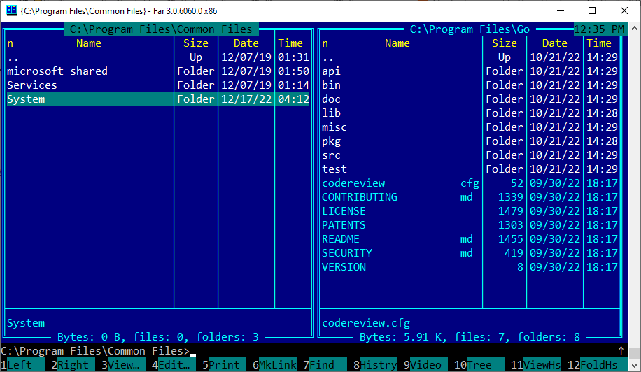
Far manager is a terminal-based file manager for Windows.

Far manager screen

Links

Basic commands

  • Tab - jump between left and right panels
  • F5 - Copy file under cursor/selection to the opposite panel
  • F6 - Move file under cursor/selection to the opposite panel
  • Shift-F5 - Create copy of a file file in the same panel
  • Shift-F6 - Rename current file
  • Enter - open file
  • Shift+arrows up/down - select files
  • F3 - View file under cursor
  • F4 - Edit file under cursor

Good parts

  • Good out of the box support for a large variety of archives
  • Free

Bad parts

  • Works only on Windows, because uses Win API
  • Current Major version of Far Manager is 3. Version 2 was far more lightweight
  • Now it hasn’t an option for turning on “Black and white” colorscheme.
  • Ugly default “Blue” color that makes you sick

More articles

Execute commands in nano

In nano, it’s trivial to execute command and paste command’s output to the current buffer. That’s what Ctrl-t does.

So, for example, you want to insert list of files with specified name. you can do this in a such way:

  • Ctrl-t
  • type ls -l | grep emacs, press Enter

How to filter rows in nano editor

We can pass text in the current buffer as input to a pipe that will pass it to another program. To do this, press Alt-\ before typing command to execute.

For example, it’s very handy to filter rows. Imagine you have these rows in your buffer:

emacs
some string
I love emacs
I hate vim
I use web-mode for emacs to write html

To leave only strings that contain word “emacs”:

  • Alt-t
  • Alt-\
  • type grep emacs
  • Enter

After that buffer will conain filtered rows:

emacs
I love emacs
I use web-mode for emacs to write html

Nano editor

Nano is the editor that can save your life if you don’t know vim, but have to do some text editing. It’s more easy to learn, and now it’s available on many linux systems.

                :::                           The
  iLE88Dj.  :jD88888Dj:
.LGitE888D.f8GjjjL8888E;        .d8888b.  888b    888 888     888
iE   :8888Et.     .G8888.      d88P  Y88b 8888b   888 888     888
;i    E888,        ,8888,      888    888 88888b  888 888     888
      D888,        :8888:      888        888Y88b 888 888     888
      D888,        :8888:      888  88888 888 Y88b888 888     888
      D888,        :8888:      888    888 888  Y88888 888     888
      D888,        :8888:      Y88b  d88P 888   Y8888 Y88b. .d88P
      888W,        :8888:       "Y8888P88 888    Y888  "Y88888P"
      W88W,        :8888:
      W88W:        :8888:      88888b.   8888b.  88888b.   .d88b.
      DGGD:        :8888:      888 "88b     "88b 888 "88b d88""88b
                   :8888:      888  888 .d888888 888  888 888  888
                   :W888:      888  888 888  888 888  888 Y88..88P
                   :8888:      888  888 "Y888888 888  888  "Y88P"
                    E888i
                    tW88D

Links

Basic usage

To run nano, type nano in a terminal.

At the bottom there’re hints for some commands you can use. ^K means Ctrl-k.

Some other commands:

  • Ctrl-r: open file
  • Ctrl-o: write content to a file (autocomplete works on Tab press)
  • Alt-u: Undo
  • Alt-r: Redo
  • Ctrl-k: Kill line or selection
  • Ctrl-k: Paste
  • Ctrl-n: Cursor down
  • Ctrl-p: Cursor up
  • Ctrl-b: Cursor left
  • Ctrl-f: Cursor right


Audit techniques in RDBMS

This article will tell you about some techniques that can help you to track changes which were performed on database tables. It is recommended to know SQL basics to understand some queries examples that are shown here, so if you are unfamiliar with SQL, you can read a simple SQL tutorial for beginners.

Why is audit needed?

Audit is the thing that is required rarely, but you can’t guess when exactly you will need it, and because of this you need to track changes all the time. The most general tasks that audit serves for are:

  • Detect what changes were performed
  • Restore previous versions of rows in tables
  • Logging user activity. Audit data can be used for analytic purposes as telemetry dataset.How often some specific user updates some specific table? What operating system or executable module he uses more often or during some specific period of time? What kind of data is changed by users more often, and so on. All these questions can be answered by researching audit data.

Additional columns

The most simple way that you can do to be able to track changes on tables is to add columns that will store info about data modifications, like when a row was created, who created it, when the row was modified last time and by whom.

It looks like this:

order_no order_cost status create_date create_user last_modified user_modified
1 1.99 7 2021-01-01 ann null null
2 1.89 5234 2021-01-01 johndoe 2021-01-28 admin

In addition to the basic columns, there are also a few audit columns: create_datecreate_userlast_modified and user_modified.

We can see that the row with order_no = 1 was created by the user ann, and since its creation, the row hasn’t changed, because last_modified and user_modified columns are empty.

The create_date and create_user columns are filled with corresponding data at the moment of data insertion to the table and they shouldn’t be modified in the future. The actual implementation of such functionality depends on the database you use. In Oracle and Microsoft SQL Server it can be(and most probably, should be) implemented by using columns’ default values.

Change tables

Warning! This way is considered as an antipattern, so you should avoid it in your database.

Change tables are the tables that store audit data along with the state of the changed row, represented as single string (Let’s name this table order_audit):

user action action_date state
ann insert 2021-01-01 order_no=1;order_cost=1.99;status=7
johndoe insert 2021-01-01 order_no=2;order_cost=1.89;status=5234
ann update 2021-01-03 order_no=1;status=8
admin delete 2021-01-03 order_no=1;order_cost=1.99;status=8

Here, we can see that when a user makes any change with a table row, another one row is added to the order_audit table, where all changes that were applied to the row are aggregated into a single string. When the user deletes a row, we also log this action by aggregating the values of all columns in the row. If we want to see all changes that user ann did with the table orders, we can write a simple query, like this:

select *
from order_audit
where user = 'ann'

While this approach is much better than just a few additional columns, it has some critical disadvantages:

  • It’s very hard to track changes for individual columns or some set of them, because the state column contains all changes that were applied, and we need an additional code to fetch specific changes. Even after that it’s hard to do something with this data, because all we will have is a column name and the string representation of its value.
  • This is a direct consequence of the previous paragraph: it’s hard to get a specific change. While it’s easy in simple cases, things become bad if we have a string value that contains the same character as the character we use for separating column changes in the aggregated string. For example, a user can write text “Please call before delivery; I can be not at home” in the order notes field, and if we use a semicolon, our state string may looks like this: id=2;order_date=2021-01-01;note=Please call before delivery; I can be not at home. Such sutuations make it difficult to split string, and we need additional logic - when we generate a value for the state column or when we are fetching single changes from string, or, more probably, in both places.
  • It’s hard to get the value of a column that wasn’t changed, because it is not represented in the change string. Though, this one may be fixed by saving values of all rows in a row.
  • Since changes are represented as strings, we have to develop formatting conventions for different types, and it’s mostly about dates: how should they be represented as strings? And once picked, format should be used forever, or it will be a fucking puzzle to work with date changes( Imagine yourself trying to write some code that should work with date strings like “2022-01-01”, “01/01/2022”, “01.03.2022 23:45:00”, and it can be even not a full list of all possible formats).

Master-detail audit tables

With this approach we create one master table to handle the main info about changes in our tables and one table for changes themself. The main difference from the previous approach is that we store the value of each column in a separate row, and by doing this, we are fixing one of the main disadvantages of the previous method - finding out changes for a concrete column in a performed transaction.

Here are the examples of such structure - the audit_master table holds info about all operations that were made alongside with information about operation itself (insert, update ,delete), user, and operation type. Of course, there are other possible columns for the main audit, such as the host machine, client application and ip address, but in the sake of simplicity, we will use more compact audit metadata.

audit_master table:

id oper oper_date user table_name
1 I 2021-01-01 10:43 ann orders
2 U 2021-01-01 10:45 ann orders
3 U 2021-01-01 13:40 ann orders
4 I 2021-01-01 15:40 admin orders

audit_detail table:

id master_id column_name column_value
1 1 i 1
2 1 order_date 2021-01-01
3 1 order_cost 23
4 1 id 2
5 1 order_date 2021-01-02
6 1 order_cost 1.89

Now it’s easy to find out which columns were changed:

select *
from audit_detail ad
where ad.master_id = :paudit_id

Note that to be able to keep changes for all columns, we need to use string type for column_value column and convert all types to string type by hands. And of course we have to use formatting conventions for dates and nulls.

Shadow tables

Shadow table is a table that contains all columns that its watched table has (with the same data types), with a few additional audit columns. Unlike the first two, this solution keeps historical data for all columns, even if they were not changed. It may look redundant, but we will see soon that this is the feature of this method. So, how should it be in a database? Each table that has to be audited, has its own audit table. Before each change, we save copy of a table row into the audit table alongside with audit info, for example:

  • Operation(Insert, Update or Delete)
  • Operation date(with time, of course)
  • Who made change(username of user id)
  • Ip address

What we should save before committing changes:

  • On insert, save new inserted row
  • On update, save new updated row
  • On delete, save current row

So, for the orders table, we need to create an audit table. All audit tables must have the same naming convention, or it will be hard for other developers to find out where they can look for changes history. In our example, we will use aud_ prefix for shadow tables.

Example of the orders table:

Column Type
id number
order_num string
order_date datetime
status number

Our aud_orders table:

Column Type
aud_id number
id number
order_num string
order_date datetime
status number
operation string
operation_date datetime
username string

Here, aud_id column is the primary key for the aud_orders table, while id is the copy of corresponding column from the orders table.

Now, let’s say, we insert a new row into the orders table:

insert into orders(order_num, order_date, status)
values('12-g', 2022-01-01, 1)

This is how our tables will look after commiting this operation:

orders:

id order_num order_date status
1 12-g 2022-01-01 1

aud_orders:

aud_id id order_num order_date status operation operation_date username
1 1 12-g 2022-01-01 1 I 2022-01-01 10:48:01 johndoe

Now, if we change some columns in this row:

update orders
set status = 2
where id = 1

Our orders table will look like this:

id order_num order_date status
1 12-g 2022-01-01 2

And aud_orders table will get another one row:

aud_id id order_num order_date status operation operation_date username
1 1 12-g 2022-01-01 1 I 2022-01-01 10:48:01 johndoe
2 1 12-g 2022-01-01 2 U 2022-01-01 10:52:01 johndoe

And later, if we will be asked for restore previous state of the row, we can easily do this by fetching whole row data from the aud_orders table, something like this:

update orders o
set (o.order_date, o.order_num, o.order_status) = (
    select order_date, order_num, order_status
    from aud_orders ao
    where ao.aud_id = 1)
where id = 1

Since all columns in a shadow table have the same type as in the audited table, we don’t bother about type conversions and don’t have to remember all conventions as it would be if we were using some of the previous audit solutions, where values are converted to strings. However, there are some difficulties with getting the columns that were actually changed. To do this, we need to compare each column in both versions of a row and fetch only those that have different values. Such task may be implemented in plain SQL via analytic functions(LAG), or we can delegate this to a client side, where it can be solved with the help of the general purpose languages(javascript, java, C# etc).

When we delete our row, the orders table became empty, but the aud_orders table will get another one row that represents the whole row right before its deletion:

aud_id id order_num order_date status operation operation_date username
1 1 12-g 2022-01-01 1 I 2022-01-01 10:48:01 johndoe
2 1 12-g 2022-01-01 2 U 2022-01-01 10:52:01 johndoe
3 1 12-g 2022-01-01 2 D 2022-01-02 08:13:28 admin

Therefore, it’s easy to find out how our order looked at the moment of deletion, and probably why it was deleted. Shadow tables also allow us to list all changes for specific row in a table:

select *
from aud_orders
where id = 1

It looks very natural, like you work with the orders table itself, and this is the most powerful and convenient feature of shadow tables.

Database-related features

Some databases have their own features for auditing, and they should be preferred over any handmade solution. However, if you feel that default audit capabilities are not enough, feel free to implement your own system that will suit your needs.

Here are some links:

Should all changes be tracked?

Of course not. There is no need to keep an eye on every table like the Big Brother, but it’s also quite hard to say when to use audit and when not. Just “Listen to your soul”.

SQL tutorial

This is the small tutorial about SQL. I hope it will help you to solve problems and make it easy for you to understand SQL.

Note: Work in progress. ☜(゚ヮ゚☜)

Info for russian-speaking readers

You should checkout my website which is dedicated to Oracle SQL and PL/SQL.

What is SQL

SQL, or Structure Query Language is the main tool for interaction with relational database management systems(RDBMS).

SQL is used to:

  • Retrieve data from DB
  • Save data to DB
  • Perform changes in existing data

SQL dialects

SQL is standardized, but who cares?

There are many RDBMS, and as a rule, each of them has its differences in SQL implementation - some of them use different syntax for the same things, some of them have or have not some features, but generally, if you know one SQL dialect, it will be not so hard to switch to another dialect when it will be needed.

In this tutorial, we will use SQLite database, since it’s easy to install on most platforms, and also it supports most of the standard SQL.

SQL features

A few words about what is so special in SQL.

Unlike many other programming languages, such as Java, Pascal or JavaScript, in which programming is performed by describing how to do things, in SQL we need to describe what we need to do, or what result we want, but generally, we can’t tell the database how to achieve this result.

Why learn SQL

As told, SQL is the main tool to talk with RDBMS.

When some program or service want to get, save or change data in a database, it does this by using SQL. Even if SQL is not used directly, and for interaction with the database some framework is used(such as Hibernate in Java), under the hood this framework generates SQL, which is then passed to the database.

DML, DDL

SQL commands can be divided into two groups - DML and DDL.

Except for DML and DDL, there are also DCL and TCL groups, but we don’t touch them in this tutorial.

DML stands for Data Manipulation Language. It consists of commands which can change or retrieve already existing data. By changing we mean also insertion of new data and deletion of old data.

So, here are the list of DML commands:

  • SELECT
  • INSERT
  • UPDATE
  • DELETE
  • MERGE

Note that SELECT command also related to DML.

DDL is stands for Data Definition Language. It consists from commands which are responsible for database objects’ creation or modification.

These commands are related to DDL:

  • CREATE
  • RENAME
  • ALTER
  • DROP
  • RENAME
  • TRUNCATE
  • COMMENT

In this tutorial, we will mostly concentrate on DML commands, but we will use DDL for creating our database schema.

SQLite installation

Linux

If you Llinux system, probably SQLite is already installed.

First, try to type into terminal following command:

sqlite3 -version

If you see something like this, SQLite is already installed:

3.31.1 2020-01-27 19:55:54 3bfa9cc97da10598521b342961df8f5f68c7388fa117345eeb516eaa837balt1

To install SQLite, we should search for sqlite package. Since there are so many different Linux distributives and theirs package managers, it’s hard to tell what exactly command you need to type, but we will list instructions for most popular linux distrubutives.

Debian-based( Debian, Ubuntu, and others)

sudo apt-get install sqlite3

Fedora

sudo dnf install sqlite

Arch linux

sudo pacman -S sqlite

Windows

You can download precompiled binaries from the official site. Precompiled binaries for Linux also can be downloaded from there.

Tables

In RDMS data is stored in the tables. Tables are the key objects, with which we have to work in SQL.

Tables in the databases don’t differ much from the tables with which you already familiar from school - they consist of columns and rows. Each column in a table has its own name and type. Generally speaking, there are five types of data that we can store in the database:

  • Numbers
  • Text
  • Dates
  • Binary data(images, pdf files and so on)
  • Nothing

These types are not related to any concrete database engine. Moreover, many databases have much more types, but those types don’t bring any new kind of data that we can store - they just split each of our types into more small subtypes. For example, the Oracle database has a DATE type( accurate to seconds). Also, it has the TIMESTAMP type, which is also used to store dates, but with more precision(accurate to parts of second).

WTF is NULL?

We need to pay attention to the last item on our list. What does it mean - Nothing? We can think about it as just an empty column in a row. But the math guy who have created relational theory did not like empty columns, and he said that all columns must have a value. But in practice, we need empty columns sometimes, so database developers have created a specific value which means that columns with this value don’t have a value. And this value is NULL. We will talk about nulls later, don’t worry, anything that we need to know for now is that this value means nothingemptyno value and so on.

Database file creation

Let’s create SQLite database which we will use to keep our database structure for later use and experiments. In terminal, type following command:

sqlite3

Right after this we will see something like this:

SQLite version 3.31.1 2020-01-27 19:55:54
Enter ".help" for usage hints.
Connected to a transient in-memory database.
Use ".open FILENAME" to reopen on a persistent database.
sqlite> 

Wee see that now we are connected to in-memory database, what means that if we quit from SQLite command prompt or shutdown the computer, all our data will be lost.

What we want is to save the database to a file so we can use it later without losing our data. To do this, .save command is used:

sqlite> .save testdb.db

After execution of the above command, file named testdb.db will be created in the current directory.

To quit SQLite command interpreter, use .quit command.

Creating test schema

Let’s create our tables and fill them with test data. We will use this schema throughout the whole SQL tutorial.

Our database structure represents an imaginary shop service, which allows users to create some orders, put some items into those orders and close them. Each order can be in one of the next states: Closed and Waiting.

create table users(
    id number primary key,
	login text,
	is_active number
);

create table orders(
	id number primary key,
	user_id number,
	order_date text,
	order_num number,
	status number
);
	
create table items(
	id number,
	item_name text
);

create table order_items(
	id number,
	order_id number,
	item_id number,
	quantity number
);create table users(
    id number primary key,
	login text,
	is_active number
);


insert into users
values(1, 'JohnDoe', 1);

insert into users
values(2, 'MrWinner', 1);

insert into users
values(3, 'Alex', 1);

insert into users
values(4, 'Barbie', 1);

insert into users
values(5, 'Lisa', 1);

insert into users
values(6, 'Stone', 0);

create table items(
	id number primary key,
	item_name text,
	price number
);

insert into items
values(1, 'Microwave', 300);

insert into items
values(2, 'Mobile phone', 350);

insert into items
values(3, 'Nintendo switch', 400);

insert into items
values(4, 'TV', 1000);

insert into items
values(5, 'Laptop', 1500);

insert into items
values(6, 'Washer', 700);

create table orders(
	id number primary key,
	user_id number,
	order_date text,
	order_num number,
	status text,
	constraint orders_users_fk foreign key(user_id)
	    references users(id)
);

insert into orders
values(1, 2, '2021-10-11', 32, 'CLOSED');
	
insert into orders
values(2, 2, '2021-08-15', 230, 'WAITING');

insert into orders
values(3, 4, '2019-04-24', 39, 'CLOSED');

insert into orders
values(4, 5, '2019-04-24', 39, 'WAITING');

create table order_items(
	id number,
	order_id number,
	item_id number,
	quantity number,
	constraint order_items_order_fk foreign key(order_id)
	    references orders(id),
	constraint order_items_item_fk foreign key(item_id)
	    references items(id)
);


insert into order_items
values(1, 1, 4, 1);

insert into order_items
values(2, 1, 6, 1);

insert into order_items
values(3, 2, 5, 2);

insert into order_items
values(4, 3, 3, 4);

insert into order_items
values(5, 3, 2, 4);

Save this query to a file, named, for example, schema.sql. Now, we need to open our database file:

sqlite3 testdb.db

To execute sql script, in SQLite command prompt, we need to use command read:

sqlite> .read schema.sql

This command executes our script, but to be able to use test data later, we need to save changes back to file:

sqlite> .save

Let’s check which tables are in the database:

sqlite>.tables

Output:

items        order_items  orders       users 

So, now we have the database file, called testdb.db, which contains tables with which we will work later. In the next chapter we will look at how to retrieve information from tables and how we can save it to external file using SQLite command prompt.

Summary

  • SQL is the main language to talk with RDBMS
  • SQL consists from DDL, DML, DCL and TCL
  • There are many SQL dialects
  • Null is specific value that determines empty value
  • To create new database file, we use command sqlite3 dbfile.db
  • To execute a sql script, .read sqlfile.sql command is used
  • To save changes back to file, .save command is used
  • .tables command shows list of tables in the current database

In this chapter, we gonna look at how to retrieve data from the database.

First select

Let’s connect to our database, which we have created previously:

sqlite3 testdb.db

To select data from database tables, SELECT command is used. It is probably the most frequently usable command in SQL, and we will use this command all the time.

Let’s see what data we have in the users table:

sqlite> select *
   ...> from users;

Result:

1|JohnDoe|1
2|MrWinner|1
3|Alex|1
4|Barbie|1
5|Lisa|1
6|Stone|0

Here we have just ran our first SQL query, which retrieves all data from the users table. One important thing - a sql query is executed after the first semicolon.

Ok, we have some results, but they look very ugly. We can’t see table columns, and here is no any formatting. Before we dive into the structure of SELECT query, let’s tweak SQLite command prompt, so that query results will look more sexy.

Sqlite prompt configuration

We gonna add options for displaying column headers and for aligning columns content. To do this, we need to create a file named .sqliterc in the home directory with the following content:

.headers on
.mode column

Now, if we run our query again, result will look much better:

id          login       is_active 
----------  ----------  ----------
1           JohnDoe     1         
2           MrWinner    1         
3           Alex        1         
4           Barbie      1         
5           Lisa        1         
6           Stone       0

Select query basics

We have ran next query:

select *
from users

In this query we have just said: “Database, please, give me all rows and all columns from the users table.

In select queries, asterisk means “All columns”. If we want to retrieve some specific columns, we need to list them. Let’s get only login names:

select login
from users

If we want to select a few columns, they should be separated by comma:

select login, is_active
from users

Table aliases

It is a good practice to use aliases in SQL queries. By using table aliases, we can say from which table column should be used. Table aliases are separated by space from the table name:

select u.login, u.is_active
from users u

Now it may look like as a redundant thing, but in complex cases, table aliases make queries much, much more readable.

Table names also can be used as aliases, so if the table name is short, it is ok to use it as an alias:

select users.login, users.is_active
from users

Column aliases

Aliases can be given for selected columns, too:

select u.login user_login,
       u.is_active is_active_flag
from users

And now our query result looks like there are users_login and is_active_flag in the users table:

user_login  is_active_flag
----------  --------------
JohnDoe     1             
MrWinner    1             
Alex        1             
Barbie      1             
Lisa        1             
Stone       0             

Rows filtering

Almost always we don’t need all data in a table, we want to get rows that satisfy some conditions. For example, we may want only active users, only inactive users, users which logins start with the symbol ‘A’ and so on.

In SQL, we specify conditions in the WHERE clause:

select u.*
from users u
where u.is_active = 1
id          login       is_active 
----------  ----------  ----------
1           JohnDoe     1         
2           MrWinner    1         
3           Alex        1         
4           Barbie      1         
5           Lisa        1         

Here we have got only active users.

When using WHERE, only those rows go to the result, which satisfy all conditions.

In the WHERE clause, we can specify multiple conditions by using AND and OR keywords.

Let’s get information about users with nicknames “MrWinner” and “Lisa”:

select u.*
from users u
where u.login = 'MrWinner'
or u.login = 'Lisa'
id          login       is_active 
----------  ----------  ----------
2           MrWinner    1         
5           Lisa        1         

We have used OR to include both rows in the result.

If we use AND, the result will be empty:

select u.*
from users u
where u.login = 'MrWinner'
and u.login = 'Lisa'

That is because there are no rows in the table which have values “MrWinner” and “Lisa” at the same time.

Grouping conditions

Let’s remember school math: things between brackets are calculated first. Same thing with conditions in SQL (actually, it is boolean logic and predicate calculations, but it’s boring):

select u.*
from users u
where (is_active = 0 or login = 'Lisa') and is_active = 1

Result:

id          login       is_active 
----------  ----------  ----------
5           Lisa        1         

If we change brackets position, the result will be different:

select u.*
from users u
where is_active = 0 or (login = 'Lisa' and is_active = 1)

Result:

id          login       is_active 
----------  ----------  ----------
5           Lisa        1         
6           Stone       0         

Export data to CSV

This topic is exclusively about the SQLite database feature. It allows you to save query results into a CSV file.

Here is the how-to:

  1. Turn on CSV mode:

    sqlite> .mode csv
    
  2. Set output file:

    sqlite> .output result.csv
    

    Here result.csv is the output file. It can has any other name.

  3. Execute query:

    qlite> select *
       ...> from users;
    

Our result csv file now contains:

id,login,is_active
1,JohnDoe,1
2,MrWinner,1
3,Alex,1
4,Barbie,1
5,Lisa,1
6,Stone,0

Additional info about command-line features of SQLite can be found at Official docs.

Summary

  • To filter query results, WHERE clause is used
  • To change the default calculation order, we can use brackets for grouping conditions
  • In SQLite, it is easy to export data into a CSV file

Sometimes we want to get result in specific order, and order by clause does exactly this.

Basic sorting

Let’s look at the data in the orders table:

select user_id, order_date, order_num
from orders
user_id     order_date  order_num 
----------  ----------  ----------
2           2021-10-11  32
2           2021-08-15  230
4           2019-04-24  39
5           2019-04-24  39 

We can retrieve orders info sorted by the order_num column:

select user_id, order_date, order_num
from orders
order by order_num asc

Result:

user_id     order_date  order_num 
----------  ----------  ----------
2           2021-10-11  32
4           2019-04-24  39
5           2019-04-24  39
2           2021-08-15  230 

As we can see, now orders are sorted by order number in ascending order. This is because we have set ascending order in the order by by adding the asc keyword.

It’s unnecessary to add asc if we want to sort rows in ascending order - it is the default. Next query is identical to the previous one:

select user_id, order_date, order_num
from orders
order by order_num

To sort rows in descending order, we should add desc to order by clause:

select user_id, order_date, order_num
from orders
order by order_num desc
user_id     order_date  order_num 
----------  ----------  ----------
2           2021-08-15  230
4           2019-04-24  39 
5           2019-04-24  39 
2           2021-10-11  32

Sorting by multiple columns

To sort rows by multiple columns, those columns should be separated by commas:

select user_id, order_date, order_num
from orders
order by user_id desc, order_date
user_id     order_date  order_num 
----------  ----------  ----------
5           2019-04-24  39
4           2019-04-24  39
2           2021-08-15  230
2           2021-10-11  32 

Here rows come sorted by userId in descending order first, and by order date in ascending order second. It is observed by the fact that rows with the same user_id(where it equals to 2) sorted by order_date in ascending order.

Sorting’s voodoo techniques

It is unnecessary for a column to be included into a select query - we can sort by column, but don’t select it at all:

select order_date, order_num, status
from orders
order by user_id desc
order_date  order_num   status 
----------  ----------  ----------
2019-04-24  39          WAITING 
2019-04-24  39          CLOSED
2021-10-11  32          CLOSED 
2021-08-15  230         WAITING

Rows are sorted by the user_id column, as in the previous example, but the user_id column itself does not exist in the result set.

We can sort columns by their order in select clause, not just by their name:

select user_id, order_date, order_num, status
from orders
order by 1, 2 desc
user_id     order_date  order_num   status
----------  ----------  ----------  ----------
2           2021-10-11  32          CLOSED 
2           2021-08-15  230         WAITING
4           2019-04-24  39          CLOSED 
5           2019-04-24  39          WAITING

The above query is the same as the next one:

select user_id, order_date, order_num, status
from orders
order by user_id, order_date desc

Such a feature can look attractive, but in practice you should avoid sorting by columns’ order, because such queries may become invalid after changing column order. Let’s demonstrate this.

Suppose we have a query:

select order_date, order_num, status
from orders
order by 1, 2 desc
order_date  order_num   status 
----------  ----------  ----------
2019-04-24  39          CLOSED 
2019-04-24  39          WAITING
2021-08-15  230         WAITING
2021-10-11  32          CLOSED 

But some time later we decide to retrieve the user_id column as well:

select user_id, order_date, order_num, status
from orders
order by 1, 2 desc
user_id     order_date  order_num   status
----------  ----------  ----------  ----------
2           2021-10-11  32          CLOSED
2           2021-08-15  230         WAITING
4           2019-04-24  39          CLOSED
5           2019-04-24  39          WAITING 

Now rows come in an absolutely different order, because the user_id column is first and the order_date is second.

Summary

  • Order by clause is used for result sorting.
  • There is no need to add asc keyword to sort rows in ascending order - this value is assumed to be the default.
  • It is the bad pattern to order rows by specifying columns order - it is better to list columns by their names.

Joins are some of the most essential concepts of SQL. They are used for querying data from multiple tables. In this article we will look at JOIN and LEFT/RIGHT JOIN - these are all what you need to know to freely work with multiple tables.

LEFT JOIN

Let’s forget about tables and databases for a while, and imagine that we have two bags with balls of various colors. Also, let’s imagine that one bag is placed on the left side and another bag is placed on the right side relating to us.

Now, let’s play the very simple game - we will take one random ball from the left bag and then we will search for all balls with the same colour in this bag. Then we search for balls with this colour in the right bag. We can write down this operation like “Find all balls of color C in bag A, and then find all balls of color C in bag B”.

In SQL, we could write a query for this:

-- Search for Red balls
select ball, colour
from A
left join B on B.colour = A.colour
where A.colur = 'Red'

We will dig deeper into examples from our test database a little bit later.

If we modify the rules a little and will take all balls from the left bag and search for all balls from the right bag with the same colour as the balls from the left bag, then we should remove the filter condition from our query:

select ball, colour
from A
left join B on B.colour = A.colour

What if we will not find any balls in the right bag, which colours match with the balls from the left bag? In this case, our result row set will contain only balls from the left bag. This is the only thing that makes JOIN and LEFT or RIGHT JOIN different.

For a concrete example, suppose we are gonna fetch info about all orders. We have the orders table, which contains info about orders, but we also want to see what items were in each order, and this info is stored in the order_items table.

First, let’s see what data lies in each of these tables:

Orders:

select *
from orders
id          user_id     order_date  order_num   status
----------  ----------  ----------  ----------  ----------
1           2           2021-10-11  32          CLOSED
2           2           2021-08-15  230         WAITING
3           4           2019-04-24  39          CLOSED
4           5           2019-04-24  39          WAITING

Order_items:

select *
from order_items
id          order_id    item_id     quantity
----------  ----------  ----------  ----------
1           1           4           1
2           1           6           1
3           2           5           2
4           3           3           4
5           3           2           4

To query data from both tables, we need to pick a condition by which these tables will be joined( like balls colors).

Here we can(and need, actually) to use order id - order_id column in the order_items table is linked to the id column in the orders table. Such relation has a corresponding specific object in databases, called “foreign key”.

So, here is our query:

select o.id, o.order_date, o.order_num, i.quantity
from orders o
left join order_items i on i.order_id = o.id
id          order_date  order_num   quantity
----------  ----------  ----------  ----------
1           2021-10-11  32          1
1           2021-10-11  32          1
2           2021-08-15  230         2
3           2019-04-24  39          4
3           2019-04-24  39          4
4           2019-04-24  39

Now let’s talk about this query in more detail. We take all rows from the orders table, and then, for every row, we take all rows from the order_items table with the same value in the order_id column. For the order with id = 4, we did not find any rows in the order_items table, so there is no value in the quantity field for this row.

RIGHT JOIN

If we will take balls from the right bag first and then search for similar colours in the left bag, this will be called RIGHT JOIN operation.

JOIN

As was said, JOIN is the operation that leaves only those rows which exist in both tables. Let’s get all user orders:

select u.id, u.login, o.order_date, o.status
from users u
join orders o on o.user_id = u.id

Result:

id          login       order_date  status
----------  ----------  ----------  ----------
2           MrWinner    2021-10-11  CLOSED
2           MrWinner    2021-08-15  WAITING
4           Barbie      2019-04-24  CLOSED
5           Lisa        2019-04-24  WAITING

Note that users with id = 1 and 2 did not appear in a result, because they do not have any orders.

Or, let’s rewrite the example from the LEFT JOIN part, but this time we will use JOIN:

select o.id, o.order_date, o.order_num, i.quantity
from orders o
join order_items i on i.order_id = o.id

Result:

id          order_date  order_num   quantity
----------  ----------  ----------  ----------
1           2021-10-11  32          1
1           2021-10-11  32          1
2           2021-08-15  230         2
3           2019-04-24  39          4
3           2019-04-24  39          4

Row with empty quantity disappeared, because there is no such row in the order_items table, where order_id is equal 4.

Using joins with more than two tables

When we want to join more than two tables, we just apply join rules for the first two tables first, then we join result of this join with third table then result is joined with the fourth table and so on.

select u.id,
       u.login,
       o.order_date,
       i.item_name,
       oi.quantity
from users u
join orders o on o.user_id = u.id
left join order_items oi on oi.order_id = o.id
left join items i on i.id = oi.item_id
where u.is_active = 1

Result:

id          login       order_date  item_name   quantity
----------  ----------  ----------  ----------  ----------
2           MrWinner    2021-10-11  TV          1
2           MrWinner    2021-10-11  Washer      1
2           MrWinner    2021-08-15  Laptop      2
4           Barbie      2019-04-24  Mobile pho  4
4           Barbie      2019-04-24  Nintendo s  4
5           Lisa        2019-04-24

Here, the users table first joined with the orders table first. We can see what we have after this join:

select u.id, u.login, o.order_date
from users u
join orders o on o.user_id = u.id
id          login       order_date
----------  ----------  ----------
2           MrWinner    2021-10-11
2           MrWinner    2021-08-15
4           Barbie      2019-04-24
5           Lisa        2019-04-24

We see, that MrWinner has two orders (different dates, and also different order_id values), Barbie and Lisa both have one order.

Important notice: when joins are performed, all columns from both tables are available for later use in a query. They don’t have to appear in the selected columns list. In our query, for example, we used the is_active column from the users table in the where clause, but the column itself did not appear in a result set.

Next, we are jeft joining this result with the order_items table:

select u.id, u.login, o.order_date, oi.quantity
from users u
join orders o on o.user_id = u.id
left join order_items oi on oi.order_id = o.id
id          login       order_date  quantity
----------  ----------  ----------  ----------
2           MrWinner    2021-10-11  1
2           MrWinner    2021-08-15  2
4           Barbie      2019-04-24  4
5           Lisa        2019-04-24

Take a look at the row with user Lisa - it does not have a value in the quantity column. This is because there are no items in her order. And since we use left join, rows that have been produced by previous joins did not disappear.

Just to see the difference, we can rewrite this query using join instead of left join:

select u.id, u.login, o.order_date, oi.quantity
from users u
join orders o on o.user_id = u.id
join order_items oi on oi.order_id = o.id
id          login       order_date  quantity
----------  ----------  ----------  ----------
2           MrWinner    2021-10-11  1
2           MrWinner    2021-08-15  2
4           Barbie      2019-04-24  4

Here, rows, which do not have order items, have been removed from the result set.

But let’s go back to our main example. The last join is with the items table, from which we select item names.

The final part is not join, but filtering (where u.is_active = 1) - we keep only those rows, which have “1” as value of the users.is_active column (actually, no rows were removed at this step, because all users in result set is active).

Using subqueries

Instead tables, we can use subqueries in any JOIN clause (It applies not only to joins - in SQL you can use subqueries almost everywhere where tables can be used).

select u.login,
       ord.order_date,
       ord.order_num,
       ord.item_name
from users u
left join (
       select o.user_id,
              o.order_date,
              o.order_num,
              oi.quantity,
              i.item_name,
              i.price
       from orders o
       join order_items oi on oi.order_id = o.id
       left join items i on i.id = oi.item_id
       where o.status = 'CLOSED'
) ord on ord.user_id = u.id

Result:

login       order_date  order_num   item_name 
----------  ----------  ----------  ----------
JohnDoe                                       
MrWinner    2021-10-11  32          TV        
MrWinner    2021-10-11  32          Washer    
Alex                                          
Barbie      2019-04-24  39          Mobile pho
Barbie      2019-04-24  39          Nintendo s
Lisa                                          
Stone                                         

Subqueries did not explained in this tutorial yet, but here it should be clear - we wrap some query in parens, assign alias name to it(ord in our case), and use it like it is a table.

Tip: Select only those columns in subqueries, which will be used later. Here, we did not use item price column (i.price), so it must be removed. Unnecessary columns, joins and conditions in subqueries make queries more complicated and harder to read later, especially for other people.

More on conditions in joins

Compound conditions

We can use compound conditions by which we are going to join tables:

select u.login, o.order_num, o.status
from users u
left join orders o on o.user_id = u.id and o.status = 'CLOSED'

Result:

login       order_num   status    
----------  ----------  ----------
JohnDoe                           
MrWinner    32          CLOSED    
Alex                              
Barbie      39          CLOSED    
Lisa                              
Stone                             

Here, only those rows from the orders table are attached to rows from the users table, where not only user_id has matched rows, but also rows that have status ‘CLOSED’.

Be careful here - it is the join condition, and it affects only on joined rows - not on a whole result. Compare query above with this one and see the difference:

select u.login, o.order_num, o.status
from users u
left join orders o on o.user_id = u.id
where o.status = 'CLOSED'

Result:

login       order_num   status    
----------  ----------  ----------
MrWinner    32          CLOSED    
Barbie      39          CLOSED    

Conditions in a where clause are applied to a whole dataset which is result of all joins in a query.

You can use any condition you want

You don’t have to join by id columns or something like that. Yes, usually, joins are performed by linking rows in one set to rows in another set by matching some columns, but it is not necessary. Join conditions are like all other conditions in SQL - they are just a rule, or set of rules, which can be evaluated to true or false, and nothing more.

For example:

select u.id, u.login, o.user_id, o.order_num
from users u
join orders o on (1 = 1)

Boom:

id          login       user_id     order_num 
----------  ----------  ----------  ----------
1           JohnDoe     2           32        
1           JohnDoe     2           230       
1           JohnDoe     4           39        
1           JohnDoe     5           39        
2           MrWinner    2           32        
2           MrWinner    2           230       
2           MrWinner    4           39        
2           MrWinner    5           39        
3           Alex        2           32        
3           Alex        2           230       
3           Alex        4           39        
3           Alex        5           39        
4           Barbie      2           32        
4           Barbie      2           230       
4           Barbie      4           39        
4           Barbie      5           39        
5           Lisa        2           32        
5           Lisa        2           230       
5           Lisa        4           39        
5           Lisa        5           39        
6           Stone       2           32        
6           Stone       2           230       
6           Stone       4           39        
6           Stone       5           39    

This is called “Decart multiplication”, or “cartesian product”.

Here, for each row in the users table, join condition is evaluated to True for all rows in the orders table. In SQL, there is special syntax for such kind of joins - CROSS JOIN. Next query is identical to the previous one:

select u.id, u.login, o.user_id, o.order_num
from users u
cross join orders o

Summary

  • Joins allow us to query data from multiple tables
  • We can join subqueries
  • Join conditions can be complex

UNION, EXCEPT, INTERSECT

In this chapter, we will look at so-called Set operators, which work with the datasets returned by two queries.

To make examples more understandable, we will create the guest_orders table, which will store orders that were placed by guest users.

Our first step is to open our testdb.db file:

sqlite3 testdb.db

Then, we need to run this query:

create table guest_orders(
    login text,
    order_date text,
    order_num,
    status text
);

insert into guest_orders
values('Anonymous', '2021-11-04', '238', 'CLOSED');

insert into guest_orders
values('JohnDoe', '2021-11-04', '239', 'CLOSED');

insert into guest_orders
values('JohnDoe', '2021-11-19', '254', 'WAITING');

insert into guest_orders
values('Alex', '2021-12-14', '283', 'WAITING');

insert into guest_orders
values('Stone', '2021-12-14', '290', 'CLOSED');

That is it. No further actions are required. When we open the testdb.db file again, it will already contain this table.

UNION

Let’s say we want to do some analytic research, and for this, we need the logins of all users who have placed the orders (without taking into account order statuses).

We already can get all logins of guest users:

select login
from guest_orders;
login    
---------
Anonymous
JohnDoe  
JohnDoe  
Alex     
Stone

As all logins of the registered users that specified in the orders table:

select u.login
from orders o
join users u on u.id = o.user_id;
login   
--------
MrWinner
MrWinner
Barbie  
Lisa    

The UNION operator combines results from two queries and removes any duplicate rows so that each row in the result set is unique:

select login
from guest_orders

UNION

select u.login
from users u
join orders o on o.user_id = u.id

Result:

login    
---------
Alex     
Anonymous
Barbie   
JohnDoe  
Lisa     
MrWinner 
Stone    

It will be easier to understand how the UNION operator works if we run each query separately:

First query:

select login
from guest_orders
login    
---------
Anonymous
JohnDoe  
JohnDoe  
Alex     
Stone    

Second query:

select u.login
from users u
join orders o on o.user_id = u.id
login   
--------
MrWinner
MrWinner
Barbie  
Lisa  

If we mix all logins, we will get this:

Anonymous
JohnDoe  
JohnDoe  
Alex     
Stone    
MrWinner
MrWinner
Barbie  
Lisa  

Now, if we remove all duplicate rows, we will get the original result. This is how the UNION operator works - getting all data and removing all duplicates, nothing complicated.

Now, get prepared for the main rule of all set operators: each query must return the same number of columns:

select item_name, id
from items

UNION

select item_id
from order_items;

We will get the error message from SQLite: Error: SELECTs to the left and right of UNION do not have the same number of result columns. There is no need for any explanations, I think.

UNION ALL

The UNION ALL operator works like the UNION operator, except that it doesn’t remove duplicates:

select login
from guest_orders

UNION ALL

select u.login
from users u
join orders o on o.user_id = u.id

Result:

Anonymous
JohnDoe  
JohnDoe  
Alex     
Stone    
MrWinner
MrWinner
Barbie  
Lisa  

Info: If you know that there are no duplicates in both queries, use the UNION ALL operator, so that a database will not spend time removing them.

EXCEPT

Let’s get the items that don’t appear in any order:

select id
from items

except

select item_id
from order_items;

Result:

id
--
1 

Yeah, just one item. Anyway, the EXCEPT operator returns unique rows from the first query, which don’t exist in the second query.

The Except operator works with two datasets, which are select queries. They can be both simple queries, as in our example, and very complex ones, but they are always just the select queries, nothing more.

What a developer must care about is the columns’ order. It may turn out that in some query he implied one meaning for the column, while in the second query he did a mistake and specified a column with a completely different sense for the same position. Such a situation is worse than an exception, because it’s easy to miss wrong results, and it’s just the time bomb.

Let’s demonstrate such a situation. Suppose we want to get all users that haven’t created any order, and we write this query:

select id, login
from users
except
select o.id, u.login
from orders o
join users u on u.id = o.user_id;

Result:

id  login  
--  -------
1   JohnDoe
3   Alex   
4   Barbie 
5   Lisa   
6   Stone  

Looks good, but it is the incorrect result. The problem here is that in the second query we fetch order id, while we need to get user id. Since both are numbers, it is easy to interpret this result as the right one.

This is the corrected query:

select id, login
from users
except
select o.user_id, u.login
from orders o
join users u on u.id = o.user_id;

Result:

id  login  
--  -------
1   JohnDoe
3   Alex   
6   Stone 

INTERSECT

The INTERSECT operator is reversed EXCEPT: It returns unique (as all set operators) rows that both exist in the first and the second query.

The following SQL statement returns the logins that appear both in the guest_orders and users tables:

select login
from guest_orders

intersect

select login
from users;

Result:

login
-------
Alex
JohnDoe
Stone

Subqueries

Subqueries are just the SQL queries that are parts of another SQL query.

Subqueries in a select clause

We can wrap any query in parentheses and put it in a select list alongside with ordinary columns:

select id,
       order_date,
       (select sum(quantity) from order_items) items_cnt
from orders o;

Note that subqueries that are placed in a select clause should return only one row and one column or return no data at all. The next query is illegal:

select id,
       order_date,
       (select oi.order_item, oi.id from order_items oi) items_cnt
from orders o;

Correlated subqueries

Correlated subqueries are the queries that use data from external (relating to them) queries:

select id,
       order_date,
       (select sum(i.quantity) from order_items i where i.order_id = o.id) items_cnt
from orders o;

Result:

id  order_date  items_cnt
--  ----------  ---------
1   2021-10-11  2        
2   2021-08-15  2        
3   2019-04-24  8        
4   2019-04-24          

For each fetched row from the orders table, the subquery is executed, and every time it will use the value of o.id column, which it takes from the “outer” query.

Subqueries as tables

We can use subqueries anywhere in a SELECT query where we can use tables. For example:

select o.id,
       i.item_name,
       ord_items.quantity
from orders o
join (
    select oi.order_id,
           oi.item_id,
           oi.quantity
    from order_items oi
    where quantity >= 2
) ord_items on ord_items.order_id = o.id
join items i on i.id = ord_items.item_id

Result:

id  item_name        quantity
--  ---------------  --------
2   Laptop           2       
3   Nintendo switch  4       
3   Mobile phone     4    

In the example above, we have joined the orders table with the subquery instead of a table. Then, we treat its data like if it’s contained in a some table with the ord_items alias.

Here is another example, where we use a subquery as a single source of data:

select a.*
from (
    select *
    from items
) a
where a.price < 500

Result:

id  item_name        price
--  ---------------  -----
1   Microwave        300  
2   Mobile phone     350  
3   Nintendo switch  400

Applying all above rules we can nest one subquery into another:

select id,
       order_date,
       status,
       login,
       qty
from (
select ord_info.id,
       ord_info.order_date,
       ord_info.status,
       ord_info.login,
       (
           select sum(oi.quantity)
           from order_items oi
           where oi.order_id = ord_info.id
       ) qty
from (
    select o.id, o.order_date, o.status, u.login
    from orders o
    join users u on u.id = o.user_id
) ord_info
) summary;

Result:

id  order_date  status   login     qty
--  ----------  -------  --------  ---
1   2021-10-11  CLOSED   MrWinner  2  
2   2021-08-15  WAITING  MrWinner  2  
3   2019-04-24  CLOSED   Barbie    8  
4   2019-04-24  WAITING  Lisa  

Here we have used the correlated subquery to get items quantity for each order, while data about orders has been obtained by joining two tables - orders and users (and this join has been performed in the subquery). Then, we have wrapped the whole query into one single subquery and have used it like it’s a table. Logically, we can imagine the query above like the next one:

select id,
       order_date,
       status,
       login,
       qty
from summary;

Where the summary table is our big outer subquery:

select ord_info.id,
       ord_info.order_date,
       ord_info.status,
       ord_info.login,
       (
           select sum(oi.quantity)
           from order_items oi
           where oi.order_id = ord_info.id
       ) qty
from orders_info ord_info

While the orders_info table can be disassembled into this:

select o.id, o.order_date, o.status, u.login
from orders o
join users u on u.id = o.user_id

Thus, subqueries can be used as build blocks for a more complex query, making it easy to write and understand.

SQL puzzle: Calendar

Found an interesting SQL puzzle: Calendar of Current Year. Here is my solution. Most probably this query may be tuned to more readable solution, but anyway, it is seemed to work.

Actually, there is one big bug - calendar headers are hard-coded. It was more correct to generate such string on the fly, with taking into account database language settings, but I am too lazy to do this.

Also, I think that original solution is kind of cheaty - it uses SQLPlus formatting settings, while query below generates string rows :)

-- Created: 2021/06/16
select cal_row
from (

select 
       case 
           when a.start_month_flag = 1 then rpad(to_char(a.mnth, 'month'), 15, ' ')
           else rpad(' ', 15, ' ')
        end || a.cal_row cal_row,
        a.mnth,
        a.rn, 
        0 flag
from (

select a.*,
       case
           when lag(a.mnth) over (order by a.week_flag, a.rn) <> a.mnth or lag(a.mnth) over (order by a.week_flag, a.rn) is null then 1
           else 0
       end start_month_flag,
              case
           when lag(a.mnth) over (order by a.week_flag, a.rn) <> a.mnth or lag(a.mnth) over (order by a.week_flag, a.rn) is null then a.rn
           else null
       end start_month_rn
from (
select a.week_flag, a.mnth, min(a.dw), lpad(listagg(a.dd, ' ') within group(order by a.dt), length(listagg(a.dd, ' ') within group(order by a.dt)) + (min(a.dw) - 1) * 2 + min(a.dw) - 1, ' ') cal_row,
      row_number() over (order by week_flag) rn
from (

select case
           when a.cal_week_flag is not null then a.cal_week_flag
           else last_value(a.cal_week_flag ignore nulls) over (order by dt) 
       end week_flag,
       --to_char(a.dm, 'month') mnth,
       trunc(dm, 'mm') mnth,
       a.* 
from (
select dm,
       dw,
       dt,
       dy,
       dd,
       case
           when lag(dw) over (partition by trunc(dm, 'mm') order by dt) is null or dw = 1 then rownum
           else null
       end cal_week_flag
from (
select trunc(a.ds + level - 1) dm, to_char(a.ds + level - 1, 'd') dw,  a.ds + level - 1 dt, lpad(extract(day from a.ds + level - 1), 2, '0') dd, to_char(a.ds + level - 1, 'dy') dy
from (
    select trunc(sysdate, 'yyyy') ds
    from dual
) a
connect by level <= add_months(trunc(sysdate, 'yyyy'), 12) - trunc(sysdate, 'yyyy')
)) a
)a
group by a.week_flag, a.mnth) a)a


union all

select 


       case when mod(level , 2) = 1 then 'Month          Su Mo Tu We Th Fr Sa'
       else '-------------- -- -- -- -- -- -- --'
       end cal_row, 
       add_months(trunc(sysdate, 'yyyy'), round(level / 2) - 1) mnth,
       case when mod(level , 2) = 1 then -1
       else 0 end rn,
        -1 flag
from dual
connect by level <= 24
)a 
order by a.mnth, flag, rn

Result:

Month          Su Mo Tu We Th Fr Sa
-------------- -- -- -- -- -- -- --
january                       01 02
               03 04 05 06 07 08 09
               10 11 12 13 14 15 16
               17 18 19 20 21 22 23
               24 25 26 27 28 29 30
               31
Month          Su Mo Tu We Th Fr Sa
-------------- -- -- -- -- -- -- --
february          01 02 03 04 05 06
               07 08 09 10 11 12 13
               14 15 16 17 18 19 20
               21 22 23 24 25 26 27
               28
Month          Su Mo Tu We Th Fr Sa
-------------- -- -- -- -- -- -- --
march             01 02 03 04 05 06
               07 08 09 10 11 12 13
               14 15 16 17 18 19 20
               21 22 23 24 25 26 27
               28 29 30 31
Month          Su Mo Tu We Th Fr Sa
-------------- -- -- -- -- -- -- --
april                      01 02 03
               04 05 06 07 08 09 10
               11 12 13 14 15 16 17
               18 19 20 21 22 23 24
               25 26 27 28 29 30
Month          Su Mo Tu We Th Fr Sa
-------------- -- -- -- -- -- -- --
may                              01
               02 03 04 05 06 07 08
               09 10 11 12 13 14 15
               16 17 18 19 20 21 22
               23 24 25 26 27 28 29
               30 31
Month          Su Mo Tu We Th Fr Sa
-------------- -- -- -- -- -- -- --
june                 01 02 03 04 05
               06 07 08 09 10 11 12
               13 14 15 16 17 18 19
               20 21 22 23 24 25 26
               27 28 29 30
Month          Su Mo Tu We Th Fr Sa
-------------- -- -- -- -- -- -- --
july                       01 02 03
               04 05 06 07 08 09 10
               11 12 13 14 15 16 17
               18 19 20 21 22 23 24
               25 26 27 28 29 30 31
Month          Su Mo Tu We Th Fr Sa
-------------- -- -- -- -- -- -- --
august         01 02 03 04 05 06 07
               08 09 10 11 12 13 14
               15 16 17 18 19 20 21
               22 23 24 25 26 27 28
               29 30 31
Month          Su Mo Tu We Th Fr Sa
-------------- -- -- -- -- -- -- --
september               01 02 03 04
               05 06 07 08 09 10 11
               12 13 14 15 16 17 18
               19 20 21 22 23 24 25
               26 27 28 29 30
Month          Su Mo Tu We Th Fr Sa
-------------- -- -- -- -- -- -- --
october                       01 02
               03 04 05 06 07 08 09
               10 11 12 13 14 15 16
               17 18 19 20 21 22 23
               24 25 26 27 28 29 30
               31
Month          Su Mo Tu We Th Fr Sa
-------------- -- -- -- -- -- -- --
november          01 02 03 04 05 06
               07 08 09 10 11 12 13
               14 15 16 17 18 19 20
               21 22 23 24 25 26 27
               28 29 30
Month          Su Mo Tu We Th Fr Sa
-------------- -- -- -- -- -- -- --
december                01 02 03 04
               05 06 07 08 09 10 11
               12 13 14 15 16 17 18
               19 20 21 22 23 24 25
               26 27 28 29 30 31